Knuth-Morris-Pratt Algorithm Explained
Tweet- Introduction
- Naive Algorithm
- KMP Algorithm
- Idea 1 : Longest Prefix Suffix
- Efficiently Computing N
- Idea #2
- Performance
- Conclusion
Introduction
Finding a substring in a string is a very common operation. People have thought of various ways to do this efficiently. In this article we will go through one of the efficient algorithms for this. This algorithm is due to Knuth Morris Pratt and is known as KMP algorithm. Before diving into this algorithm lets establish some conventions and also look at how naive substring search would work.
Naive Algorithm
In this article we would assume that variable denoted by upper case T holds the text which we want to search and upper case P holds the pattern we want to search. Also, we use integer enclosed in square brackets to refer to individual character in the text or pattern. This integer is also called index. e.g. First character in text or pattern is refered using T[0] or P[0], which indicates that the indices start a zero rather than one. This choice of 0 based index is common in programming languages. We also use SUBSTRING(S,START, END) which returs a substring of S starting from character at S[START] and ending at character S[END]. Note that both START and END are inclusive. This is different from programming languages where END is exclusive.
In the Naive algorithm we match each character in P with each character in T sequentially starting from p[0] and T[0] and if there is a failure we repeat the process starting from T[1] and if there is failure again then at T[2] and so on.
Let us look at an example of each to understand it fully. For example, we take T="babcbabcabcaabcabcabcacabc" and P="abcabcacab". Following is this simple algorithm implemented using python
# searches pattern P in text T
# returns -1 if pattern is not found
def search(P,T):
    p=0
    t=0
    while t < len(T):
        # save the starting position of t
        tstart = t
        while t < len(T) and p < len(P) and T[t] == P[p]:
            t = t + 1
            p = p + 1
        # if we matched entire pattern
        # return match position
        if p == len(P):
            return t - len(P)
        # begin search at next
        # position in T
        t = tstart + 1
        # we start matching pattern from start
        # at new position in T
        p = 0
    return -1
Following is the trace of all character comparisons made by this algorithm. In total we make 47 comparisons. We compare pattern at each position in T starting from 0 as long as we match characters. In case there is a mismatch we restart matching the pattern at next location in T.

As is evident in above trace we match many characters in T multiple time. For example, we match T[12] 4 times at step 6,9,12 and 13. Except T[0], T[1], T[5],T[20],T[21],T[22],T[23],T[24] we match all other characters at least twice. Also, in pattern we match P[0] 16 times and P[1] 6 times, we also match others characters in P multiple times. Also, in each step we forget characters we looked at in previous steps and start the search all over again from P[0]. The KMP algorithm improves upon this by utilizing the information from previous steps so that it can minimize number of repeated matches. Also, notice how in step 7, we start the search at T[6] whereas in previous step we already looked at characters in T from T[5] to T12]
KMP Algorithm
In previous section we looked at the naive algorithm and we compare pattern as long as it matches and when there is a mismatch the search is started at p=0 in P and t=tstart + 1 in T at each step and if there is no mismatch and pattern is exhausted we return the position in T from where we starting comparing.
Overall structure of KMP algorithm is also similar but with a difference . In KMP algorithm instead of starting next step at t=tstart +1, p=0 we use a lookup table which tells as where to restart the search when there is a mismatch. Lets say that table is stored in variable N and this table has one entry for each position in P i.e. len(N) == len(P). Using this table KMP search algoritm looks as follows.
# searches pattern P in text T
# returns -1 if pattern is not found
def search(P,T):
    p=0
    t=0
    while t < len(T):
        # save the starting position of t
        tstart = t
        while t < len(T) and p < len(P) and T[t] == P[p]:
            t = t + 1
            p = p + 1
        # if we matched entire pattern
        # return match position
        if p == len(P):
            return t - len(P)

        # again compare the current character in T
        # except when N[p] is -1. if N[p]=-1 no need
        # compare current character
        t = t if N[p] != -1 else t + 1

        # calculate new pattern
        # to match using N table
        p = N[p] if N[p] != -1 else 0
    return -1
Now all that is remaining is to calculate N. The table N can be calculated using pattern P alone. i.e. table has no knowledge of the text T and it can be used to find pattern P in any text. There are couple of ideas we need to understand in order to calculate N
Idea 1 : Longest Prefix Suffix
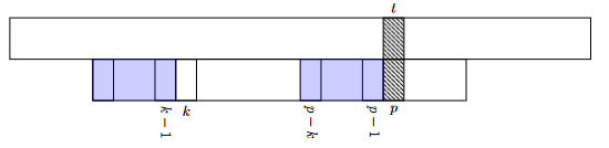
Now in order to understand construction of N let’s consider the state of algorithm above when we find a mismatch. Let’s say find mismatch in T at position t and in P at p. i.e. we found that T[t] != P[p]. Now this also means that characters in SUBSTRING(T,t-p,t-1) matched the substring in pattern SUBSTRING(P,0,p-1). Given this, if k is the largest integer such that k < p and SUBSTRING(P,0,k-1) == SUBSTRING(P,p-k,p-1) then next T[t] should be compared with P[k]. In other words if we can find largest proper prefix of pattern of length k which is also a suffix at P[p-1], then instead of falling back to matching P[0] to T[tstart+1] as we did in naive approach, we need not match any character earlier than T[t] and earlier than P[k]. Following two points must be highlighted while caluating N.
- T prefix has to be a proper prefix because of the condition
k<pas ifk=pthen we would be matching same characterP[p]. kand the prefix has to be largest such prefix.
Also, Following table illustrates calulation of N using this definition.
Position p |
Pattern | Suffixes at p-1 | Proper Prefixes | Largest Suffix/Prefix | Length k |
Comments |
|---|---|---|---|---|---|---|
| 0 | a | ”” | N/A | N/A | -1 | No prefix of lenth < p is possible when p=0 |
| 1 | ab | ”“,a | ”” | ”” | 0 | |
| 2 | abc | ”“,b,ab | ”“,a | ”” | 0 | |
| 3 | abca | ”“,c,bc,abc | ”“,a,ab | ”” | 0 | |
| 4 | abcab | ”“,a,ca,bca,abca | ”“,a,ab,abc | a | 1 | |
| 5 | abcabc | ”“,b,ab,cab,bcab,abcab | ”“,a,ab,abc,abca | ab | 2 | |
| 6 | abcabca | ”“,c,bc,abc,cabc,bcabc,abcabc | ”“,a,ab,abc,abca,abcab | abc | 3 | |
| 7 | abcabcac | ”“,a,ca,bca,abca,cabca,bcabca,abcabca | ”“,a,ab,abc,abca,abcab,abcabc | abca | 4 | |
| 8 | abcabcaca | ”“,c,ac,cac,bcac,abcac,cabcac,bcabcac,abcabcac | ”“,a,ab,abc,abca,abcab,abcabc,abcabca | ”” | 0 | |
| 9 | abcabcacab | ”“,a,ca,aca,caca,bcaca,abcaca,cabcaca,bcabcaca,abcabcaca | ”“,a,ab,abc,abca,abcab,abcabc,abcabca,abcabcac | a | 1 |
Taking values from “Length” column from above table
N = [-1,0,0,0,1,2,3,4,0,1]
Following is the trace of KMP using above N

Total number of comparisons is down to 30 from 47 in Naive approach. Although, there are still some repeated comparisons. Some these comparisons can be avoided using second idea in KMP algorithm which we will see later in this article.
Efficiently Computing N
Now we have seen how KMP works and how it uses fewer comparisons than brute force approach. We manually calculated N using longest prefix/suffix and used it to run the algorithm. Now let us look at an algorithm to compute it.
We can use DP using following recursive relation to compute N
N[j+1] = N[j] + 1, if P[j] == P[N[j]]
This relation simply says that
SUBSTRING(P,0,N[j]-1)is longest proper prefix with lengthN[j]which is also suffix ofSUBSTRING(P,0,j-1)- and if
P[j]==P[N[j]]
then SUBSTRING(P,0,N[j]) is also longest proper prefix with length N[j] + 1 which also suffix of SUBSTRING(P,0,j)
For example, from the table previous section, for j=5
N[5] = 2
SUBSTRING(P,0,N[j]-1)  or SUBSTRING(P,0,1) == "ab"
SUBSTRING(P,0,j-1) or SUBSTRING(P,0,4) == "abcab"
since “ab” is longest prefix and suffix of “abcab”. This satisfies condition #1 above. Now,
P[5] = "c"
P[N[j]] or P[2] == "c"
This satisfies the second condition above. Therefore,
SUBSTRING(P,0,N[j]) or SUBSTRING(P,0,2) == "abc"
SUBSTRING(P,0,j) or SUBSTRING(P,0,5) == "abcabc"
since “abc” is longest proper prefix and suffix of “abcabc”. This demonstrates the conclusion.
Now we know how to calulate N[j+1] if P[j] == P[N[j]] but if P[j] != P[N[j]] we can check P[j] == P[N[N[j]]] if yes, then N[j+1] = N[N[j]] + 1
Now let see why this relation is correct, as we know that
SUBSTRING(P,0,N[j]-1) is longest prefix/suffx for SUBSTRING(P,0,j-1)
We also know that
SUBSTRING(P,0,N[N[j]] - 1) is longest prefix/suffix for SUBSTRING(P,0,N[j]-1)
Which means that
SUBSTRING(P,0,N[N[j]]-1) is also next possible logest prefix/suffix of SUBSTRING(P,0,j-1)
hence if P[j]==P[N[N[j]]] then
SUBSTRING(P,0,N[N[j]]) is also longest prefix/suffix of SUBSTRING(P,0,j)
therefore, N[j+1] = N[N[j]] + 1 if P[j]==P[N[N[j]]]
Based on above, following the method in python to calucate N
# calculate N for pattern P
def calculateN(P):
    N=[0]*len(P)
    N[0] = -1
    j=0
    N_k=N[j]
    while j < len(P) - 1:
        # if P[j] != P[N[k]]
        # we try P[N[N[k]]] and so on
        #k = j
        while N_k > -1 and P[j] != P[N_k]:
            N_k = N[N_k]

        # if there is match P[j] = P[N[k]]
        # N[j+1] = N[k] + 1
        N_k = N[j+1] = N_k + 1

        # prepare for next iteration
        j = j + 1
    return N
Idea #2
Although, we have all the pieces required for a working KMP algorithm but there is one more optimization possible when we compute N. So, far we have been saying that N[p] is length of the longest proper prefix/suffix of P[p-1]. We use value of N[p] in search algorithm when P[p] does not match T[t]. Now lets say as per N if next character to match is N[p] and if we know that P[N[p]] is same as P[p] then we know that even P[N[p]] will not match T[t]. Since, this result can be deduced soley by looking at P we can use this to further optimize calulation of N and save a comparision when we use N in search method. With this optimization N[p] is equal to largest k < p such that SUBSTRING(P,0,k-1) is suffix of SUSBSTRING(P,0,p-1) and P[p] != P[k]. So, we need to change our algorithm to incorporate this last condition.
def calculateN(P):
    N=[0]*len(P)
    N[0] = -1
    j=0
    N_k=N[j]
    while j < len(P) - 1:
        # if P[j] != P[N[k]]
        # we try P[N[N[k]]] and so on
        #k = j
        while N_k > -1 and P[j] != P[N_k]:
            N_k = N[N_k]

        # if there is match P[j] = P[N[k]]
        # N[j+1] = N[k] + 1
        N_k = N[j+1] = N_k + 1

        # Idea2 that if P[j+1] == P[N_k]
        if P[j+1] == P[N_k]:
            N[j+1] = N[N_k]

        # prepare for next iteration
        j = j + 1
    return N
The new calculated value is
N=[-1, 0, 0, -1, 0, 0, -1, 4, -1, 0]
Using above definition of N following is the trace of our search function
| Step No. | 1 | 2 | 3 | 4 | 5 | 6 | 7 | 8 | 9 | 10 |
|---|---|---|---|---|---|---|---|---|---|---|
| 1 | T[0]!=P[0] | |||||||||
| 2 | T[1]=P[0] | T[2]=P[1] | T[3]=P[2] | T[4]!=P[3] | ||||||
| 3 | T[5]=P[0] | T[6]=P[1] | T[7]=P[2] | T[8]=P[3] | T[9]=P[4] | T[10]=P[5] | T[11]=P[6] | T[12]!=P[7] | ||
| 4 | T[12]!=P[4] | |||||||||
| 5 | T[12]=P[0] | T[13]=P[1] | T[14]=P[2] | T[15]=P[3] | T[16]=P[4] | T[17]=P[5] | T[18]=P[6] | T[19]!=P[7] | ||
| 6 | T[19]=P[4] | T[20]=P[5] | T[21]=P[6] | T[22]=P[7] | T[23]=P[8] | T[24]=P[9] |
Total comparisons with new N is only 28.
Performance
Performance of KMP algorithm is O(len(T) + len(P)). Looking at searching algorithm, we can see that it contains two loops. The outer loop end when t is equal to or greater than len(T). Also, since inner loop increments t it only counts towards total execution. For example, if inner loop were to run len(T) times then outer loop would also end.
Note that we never decrement t. Although, it may happen that for some cycles we do not increment t and these cycles should add to total number of executions. So, only thing we need to do to calculate time complexity is to measure number of time we do not increment t. We do not increment t when N[p] is not -1 otherwise we increment the t. N[p] is definitely -1 at p=0. Also, notice the next line where we set p = N[p]. Since N[p] is always less than p, this step always decreases p unless p=0. Which means whenever we do not increment t we decrement p and when p=0 we increment t.
Based on above we can modify the algorithm as follows such that it has simplified structure but its runtime is worse than the original algorithm. It will allow us to calculate upper bound on number of iterations where we do not increment t
def worse_search(P,T):
   p=0
   t=0

   while t < len(T):
       # r is a random number
       t = t + r
       p = p + r
       if p == 0:
         t = t + 1
       else:
         p = p - 1
Now this function has worse time because
- We run till end of
T. In original the pattern may match earlier and function may end early - At the last line we decrement
pby only1. In original we setp=N[p].N[p]may be much smaller thanp-1 - Also, we increment
tonly whenp=0. In original,twould be incremented more often asN[p]is-1at other values ofpas well other than0
Now consider an iteration in loop when t=t1 and p=0. Now let’s say that for this iteration r=r1 and for all subsequent iterations r=0. In this case t=t+r1 will be repeated i.e. not incremented for r1 times until p=0 again. So, for example, if r=1, t1+1 value of t is repeated once, i.e. once extra loop where t is not incremented and if r=2 then t1+2 is repeated at most twice. As total value of r summed over all iterations cannot be more than len(T) (as r is also added to t and t is never decremented), total number of repeated iterations i.e. iterations where t is not incremented also cannot be more than len(T). And there we have it, the upper bound on number of iterations where t is not incremented. And we know that number of iterations where we increment t can anyway never be more than len(T). So, total time cannot be more than 2*len(T) i.e. O(len(T))
We should also include the O(len(P)) preprocessing time, which gives us O(len(T) + len(P)) total complexity of algorithm.
Conclusion
KMP is a clever pattern searching algorithm with linear time complexity. It took me while to really understand how this algorithm works and how its time complexity is linear.